1. Classification

We will begin our look at decoders by using an MEG dataset of humans performing a visual categorization task. Briefly, participants saw a list of 92 images. Here, we will only use 24 of these images, either of faces or not faces. For more information, consult MNE’s documentation or the original paper.

For convenience, we will consider only gradiometer channels from the dataset, though you are free to change this, of course. The goal will be to build a classifier that can distinguish between faces/not-faces.

First, we will have to load the data—To do this, we use MNE’s sample code. Be aware that this will download roughly 6GB of data, which may take a while.

import numpy as np
import pandas as pd
from pandas import read_csv
import matplotlib.pyplot as plt

import mne
from mne.datasets import visual_92_categories
from mne.io import concatenate_raws, read_raw_fif

print(__doc__)

data_path = visual_92_categories.data_path()

# Define stimulus - trigger mapping
fname = data_path / "visual_stimuli.csv"
conds = read_csv(fname)
print(conds.head(5))

max_trigger = 24
conds = conds[:max_trigger]  # take only the first 24 rows

conditions = []
for c in conds.values:
    cond_tags = list(c[:2])
    cond_tags += [
        ("not-" if i == 0 else "") + conds.columns[k] for k, i in enumerate(c[2:], 2)
    ]
    conditions.append("/".join(map(str, cond_tags)))
print(conditions[:10])

event_id = dict(zip(conditions, conds.trigger + 1))
event_id["0/human bodypart/human/not-face/animal/natural"]

n_runs = 4  # 4 for full data (use less to speed up computations)
fnames = [data_path / f"sample_subject_{b}_tsss_mc.fif" for b in range(n_runs)]
raws = [
    read_raw_fif(fname, verbose="error", on_split_missing="ignore") for fname in fnames
]  # ignore filename warnings
raw = concatenate_raws(raws)

events = mne.find_events(raw, min_duration=0.002)

events = events[events[:, 2] <= max_trigger]

picks = mne.pick_types(raw.info, meg=True)
epochs = mne.Epochs(
    raw,
    events=events,
    event_id=event_id,
    baseline=None,
    picks='grad',
    tmin=-0.1,
    tmax=0.500,
    preload=True,
)

   trigger       condition  human  face  animal  natural
0        0  human bodypart      1     0       1        1
1        1  human bodypart      1     0       1        1
2        2  human bodypart      1     0       1        1
3        3  human bodypart      1     0       1        1
4        4  human bodypart      1     0       1        1
['0/human bodypart/human/not-face/animal/natural', '1/human bodypart/human/not-face/animal/natural', '2/human bodypart/human/not-face/animal/natural', '3/human bodypart/human/not-face/animal/natural', '4/human bodypart/human/not-face/animal/natural', '5/human bodypart/human/not-face/animal/natural', '6/human bodypart/human/not-face/animal/natural', '7/human bodypart/human/not-face/animal/natural', '8/human bodypart/human/not-face/animal/natural', '9/human bodypart/human/not-face/animal/natural']
Finding events on: STI101
4142 events found on stim channel STI101
Event IDs: [  1   2   3   4   5   6   7   8   9  10  11  12  13  14  15  16  17  18
  19  20  21  22  23  24  25  26  27  28  29  30  31  32  33  34  35  36
  37  38  39  40  41  42  43  44  45  46  47  48  49  50  51  52  53  54
  55  56  57  58  59  60  61  62  63  64  65  66  67  68  69  70  71  72
  73  74  75  76  77  78  79  80  81  82  83  84  85  86  87  88  89  90
  91  92  93 200 222 244]
Not setting metadata
720 matching events found
No baseline correction applied
0 projection items activated
Loading data for 720 events and 601 original time points ...
0 bad epochs dropped

Now that we have succesfully loaded the data, we will quickly bring the data into a format that we can work with (i.e., arrays) and produce a vector of target labels as well:

X_nf = epochs['not-face'].get_data(picks = 'grad') # grab data from not-face epochs
X_if = epochs['face'].get_data(picks = 'grad') # grab data from face epochs

# concatenate the data to make it easy to label
# i.e., data is (trials, channels, time)
X = np.concatenate((X_nf, X_if), axis = 0)

# create labels
y = [0] * 360 + [1] * 360

# for model fitting, we want labels to match the dimensions of our data, i.e. (trials, channels, time)
y = np.array(y)[:,None,None] * np.ones((X.shape[0], 1, X.shape[-1]))

print(X.shape, y.shape)

(720, 204, 601) (720, 1, 601)

Now that we have our data in a nicely structured format, let’s look at building our classifier. We will build our classifier using torch. Consequently, we will begin by transforming our data to torch tensors. Note that, if you have a GPU, you may also specify a different device than ‘cpu’ here.

Next, we will create a relatively standard pipeline using a combination of MVPy estimators and sklearn utilities.

%%

import torch
from mvpy.estimators import Scaler, Covariance, Sliding, Classifier
from sklearn.pipeline import make_pipeline
from sklearn.model_selection import StratifiedKFold

# transform our data to torch on specified device
device = 'cpu' # if desired, change your device here
X_tr, y_tr = torch.from_numpy(X).to(torch.float32).to(device), torch.from_numpy(y).to(torch.float32).to(device)

# define our cross-validation scheme
n_splits = 5
skf = StratifiedKFold(n_splits = n_splits)

# define our classifier pipeline:
#    1. Apply a standard scaling to our data to ensure that all features are on the same scale
#    2. Compute the covariance matrix of our data and use it to whiten our data.
#    3. Create a sliding estimator that will slide a classifier over the dimension of time for us. We also specify a range of alpha values for our Classifier to test, of course.
pipeline = make_pipeline(Scaler().to_torch(),
                         Covariance(method = 'LedoitWolf').to_torch(),
                         Sliding(Classifier(torch.logspace(-5, 10, 20)),
                                 dims = torch.tensor([-1]),
                                 n_jobs = None,
                                 verbose = True))

# setup our output data structures: out-of-sample accuracy, and the patterns the classifier used.
oos = torch.zeros((n_splits, X.shape[-1]), dtype = X_tr.dtype, device = X_tr.device) # (folds, time points)
patterns = torch.zeros((n_splits, X.shape[1], X.shape[-1]), dtype = X_tr.dtype, device = X_tr.device) # (folds, channels, time points)

# loop over cross-validation folds
for f_i, (train, test) in enumerate(skf.split(X_tr[:,0,0], y_tr[:,0,0])):
    # fit model
    pipeline.fit(X_tr[train], y_tr[train])

    # score model
    y_h = pipeline.predict(X_tr[test])
    oos[f_i] = (y_h[:,None,:] == y_tr[test]).to(torch.float32).mean((0, 1))

    # obtain pattern
    pattern = pipeline[2].collect('pattern_')
    pattern = torch.linalg.inv(pipeline[1].whitener_) @ pattern
    pattern = pipeline[0].inverse_transform(pattern[:,:,0].T[None,:,:])
    patterns[f_i] = pattern.squeeze()

Fitting estimators...:   0%|          | 0/601 [00:00<?, ?it/s]
Fitting estimators...:   0%|          | 0/601 [00:10<?, ?it/s]

Fitting estimators...:   0%|          | 0/601 [00:00<?, ?it/s]
Fitting estimators...:   0%|          | 0/601 [00:10<?, ?it/s]

Fitting estimators...:   0%|          | 0/601 [00:00<?, ?it/s]
Fitting estimators...:   0%|          | 0/601 [00:09<?, ?it/s]

Fitting estimators...:   0%|          | 0/601 [00:00<?, ?it/s]
Fitting estimators...:   0%|          | 0/601 [00:10<?, ?it/s]

Fitting estimators...:   0%|          | 0/601 [00:00<?, ?it/s]
Fitting estimators...:   0%|          | 0/601 [00:10<?, ?it/s]

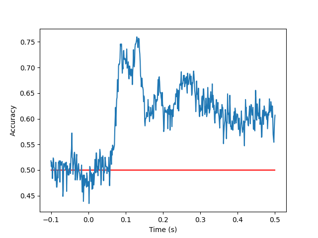
Once we have fit our model, we may now wish to look at how well it performed. Let’s do so now.

fig, ax = plt.subplots()
t = np.arange(-0.1, 0.5 + 1e-3, 1e-3) # epochs range from -100ms to +500ms
ax.plot(t, [0.5] * oos.shape[-1], color = 'red', label = 'chance') # plot chance-level
ax.plot(t, oos.cpu().numpy().mean(axis = 0), label = 'classifier') # plot classifier performance
ax.set_ylabel(r'Accuracy')
ax.set_xlabel(r'Time (s)')

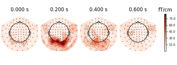
Finally, we would also like to visualise the patterns that the classifier used. Let’s visualise this briefly using MNE:

parray = mne.EpochsArray(patterns, info = epochs.info).average()
parray.plot_topomap(ch_type = "grad");

Not setting metadata
5 matching events found
No baseline correction applied
0 projection items activated